Simulating channel flows with inflow and outflow boundary conditions

🗞️ Highlights

• Our solver now supports inflow and outflow boundary conditions, allowing us to simulate two-dimensional channel flows.
• The solver is second-order accurate and matches analytical solutions.
• We have validated our simulations for the backward-facing step problem against experimental and numerical studies from the literature.
  
  

In this blog, we share a new feature of our CFD solver which enables us to simulate two-dimensional channel flows. The solver now supports inflow and outflow boundary conditions, which allows the flow to enter and leave the computational domain. Such boundary conditions are essential for simulating industrially valuable problems, most notably wind tunnels. 

Channel flow setup

As an illustrative example of these boundary conditions in action, we model a two-dimensional “channel” of fluid moving in the horizontal direction as shown in Figure 1 below. On the left of the channel, we have inflow conditions, where fluid flows to the right with an imposed velocity . On the right, we have outflow conditions, where the fluid is leaving the channel with zero normal derivative of velocity at the right boundary of the channel.

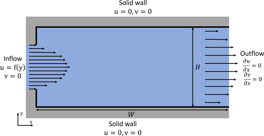
Figure 1: Setup for the channel flow problem with inflow-outflow boundary condition

Hagen-Poiseuille flow

We demonstrate the accuracy of our solver with inflow-outflow boundary conditions by performing several numerical experiments.

In the first experiment, we consider parabolic flow through a channel of width W=2 and height H=1. The initial velocity field consists of uniform random perturbations in the range of -1 to 1. A no-slip boundary condition is applied at the top and bottom walls, while the left and right boundaries are set to have inflow and outflow conditions respectively. The inflow x-velocity at the left boundary is set as:

This is an example of Hagen–Poiseuille flow, and for low Reynolds numbers, the velocity field gradually attains a steady state, and the inflow and outflow velocity profile will be the same. Therefore, at a steady state, the analytical solution for the outflow velocity will be the inflow velocity. To achieve this result, we set the Reynolds number to 50 and ran the simulations until they reached a steady state (see Figure 2: left). In Figure 2: right, we show the results obtained from our solver and the expected velocity field given by the inflow conditions. The results show that our solver simulates the Hagen-Poiseuille accurately.

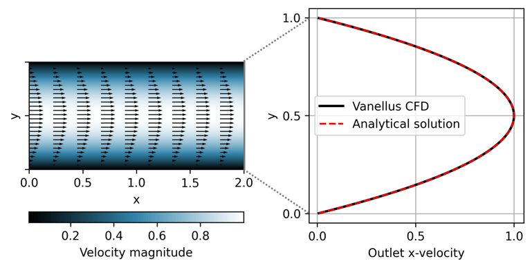
Figure 2: The velocity profile across the channel for Reynolds number = 50, with black arrows indicating the magnitude and direction of flow at selected points (left). The comparison of numerically computed velocity profiles at the outflow boundary (x = 2) with an expected analytical solution at a steady state (right).

We also conducted a convergence test of the results obtained using the Vanellus-CFD solver. Here, we performed several simulations with increasingly fine grids. The number of cells along the vertical direction is varied from 16 up to 512. The root-mean-squared-error is computed for each resolution with the 512 number of cells test as the ground truth. The results are presented in Figure 3, showing second-order convergence.

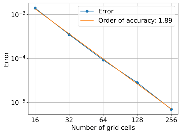Figure 3: Convergence test with increasingly fine grids to show second-order accuracy of the Vanellus-CFD solver.

Backward-facing step flow

The study of backward-facing step flow is an important test problem in fluid mechanics. This is where the fluid encounters a sudden back step causing flow separation, as depicted in Figure 4. Subsequently, the flow reattaches and recovers a parabolic profile downstream of the step. The re-circulation zone is identified as the area from the step on the left to where the flow reattaches. The point on the x-axis where the flow reattaches is the reattachment length. One of the key measures of the model's validity is the accurate prediction of this reattachment length.

The inflow conditions for the problem are applied to only a small portion of the left wall to resemble flow over a step. The inlet has a height of h=0.5, the pipe downstream has a height of H=1, and the channel has a width of W=12. The inflow x-velocity at the inlet, f(y) is given by:

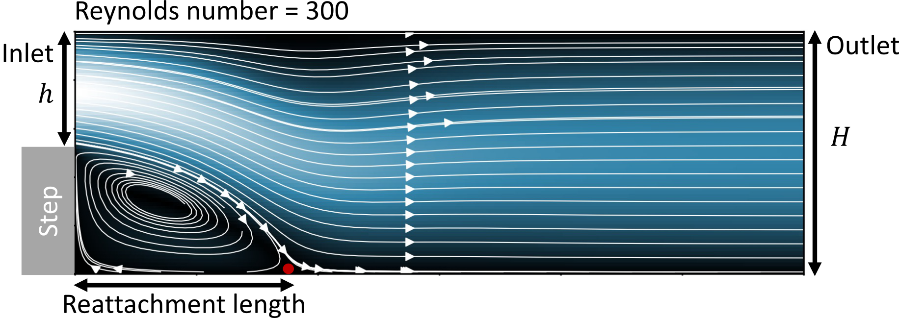
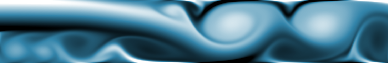
Figure 4: The velocity profile for flow over a backward-facing step at Reynolds number 300.

The publications of Armaly et al. (1983), Kim & Moin (1985) and Barton (1997) are considered the gold standard for benchmarking the backward-facing step problem. Armaly et al. (1983) presented the first experimental results for reattachment length at various Reynolds numbers, whilst the latter are numerical studies which provide data for the reattachment lengths.

Comparing our results with academic literature

Below we show a comparison of our results for normalised reattachment length at steady states computed for Reynolds numbers from 50 to 800 with literature data. 

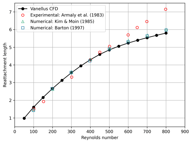Figure 6:  A comparison of the simulated reattachment length with experimental and numerical data.

From the figure above, we see that our simulation results are in good agreement with those from the previous numerical studies (Kim & Moin (1985), Barton (1997)). However, with the experimental data (Armaly et al. (1983)) our results only agree up to Reynolds number 400, as do the other numerical studies. Armaly et al. conjectured that the discrepancy between the experimental measurements and the numerical prediction was due to another re-circulation zone at the top of the channel that perturbs the two-dimensional character of the flow. Therefore this discrepancy is inherent to the fact that we are solving the 2D problem, and the real-world experiments are naturally three-dimensional.

Next steps

The validation presented here shows that our CFD solver can accurately solve problems with inflow and outflow boundary conditions. This provides a strong foundation for moving to the next stage of development, implementing embedded boundary conditions which are required for simulating airflow around objects inside wind tunnels, such as planes, cars and wind turbine blades.