Validating our differentiable fluid solver

Paving the way towards machine-learning accelerated fluid simulations.

🗞️ Highlights

• We have built a differentiable two-dimensional fluid solver from scratch which natively runs on GPUs and TPUs.
• The solver has been rigorously validated by comparing it against academic literature and industry-standard software.
• The solver’s differentiability paves the way for us to use machine learning to achieve order-of-magnitude efficiency gains.

At Vanellus, we are deploying cutting-edge machine learning research to build computational fluid dynamics (CFD) software that is dramatically more efficient than current solutions. To integrate machine learning into a CFD solver it needs to be fully differentiable, and currently no industrial-grade software supports this. Therefore, we are developing our own fluid solver from scratch, supporting differentiability and native deployment on GPUs and TPUs from day one.

In this blog, we share our recent progress in building our new solver by demonstrating its ability to accurately solve the industry-standard benchmarking problem of a lid-driven cavity.

Motivation for validating

Fluid simulations give engineers vital information on the performance of their designs prior to the expensive process of physical testing. It is therefore critical that simulations give results that are as accurate as possible given the computing resources available. Existing simulation tools such as Ansys Fluent and OpenFOAM have been used by engineers for decades and have been extensively validated. To gain the trust of engineers we aim to rigorously validate our solver as we continue to extend its functionality.

So, how do you validate a fluid solver?

The ideal form of validation is to directly test simulation results against real-world data. For example in aerodynamics, experimental data can be collected from placing a car or a wing in a wind tunnel. Unfortunately, experimental data like this is often extremely costly and difficult to obtain, requiring techniques such as particle image velocimetry to capture data on the velocity of the air in a wind tunnel.

As CFD has become ubiquitous over the last few decades, there exists a wealth of literature and software that has been benchmarked against both experimental and analytical results, proving their robustness. Therefore, to validate our software, we compare our results to those from well-trusted papers and industrial CFD software.

The lid-driven cavity problem

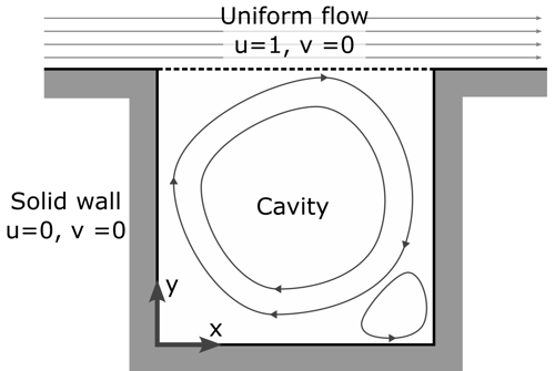
One of the most common benchmarking problems in CFD is known as the lid-driven cavity. The scenario models a two-dimensional “cavity” of fluid, which is essentially a square box with an open lid. Above the box, the fluid is flowing to the right with a constant velocity. Initially, the fluid inside the cavity is stationary and is subsequently pushed by the flow above the lid. The mathematical setup for this problem is depicted below, where “u” is the velocity of the fluid in the horizontal direction and “v” is the velocity in the vertical direction.

The lid-driven cavity problem has been one of the most popular benchmarking problems over the last fifty years, and for good reasons. For one, it is very simple to define and set up. However, despite how simple the definition of the problem seems, the resulting flow can exhibit a wealth of complex behaviour present in real-world flows, such as eddies, turbulence and flow separation. 

It is also possible to produce a real-world lid-driven cavity in a laboratory setting, as can be seen in the video from SUTD-MIT below.

How do we compare with academic literature?

The publications of Ghia et al. (1982) and Erturk et al. (2005) are considered the gold standard for benchmarking the lid-driven cavity problem. Both provide data for steady-state solutions to the lid-driven cavity problem at various Reynolds numbers (which measure the ratio between the inertial and viscous forces of the fluid). To compare our solver to this data, we ran our simulations for a long enough time to reach a steady state.

Below we show a comparison of our results to the literature data for two different Reynolds numbers. Simulating a square cavity of width 1, we compare slices of the horizontal and vertical velocities taken at the centre lines of the cavity (i.e. x = 0.5 on the left, and y = 0.5 on the right).

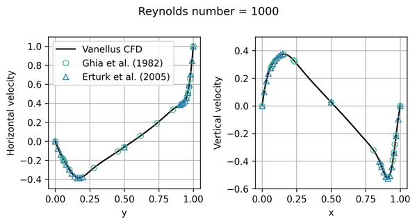
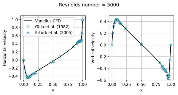
From the figure, we see that our simulation results agree well with the data taken from the literature, in particular resolving well the sharp gradients close to the walls of the cavity. This provides confidence that our solver is meeting the benchmarks set by academic literature.

How do we compare with industry-standard software?

We have demonstrated that our solver meets the benchmarks set in academia, but how does it compare to solvers used every day by engineers? We aim to compete with existing CFD software, so it is vital to compare our results to current industry standard solvers to ensure we can reproduce their level of accuracy.

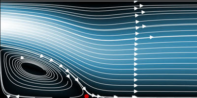
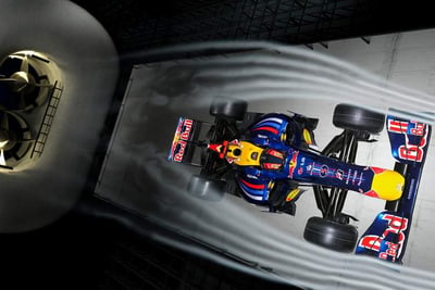
One of the leading CFD solvers used by engineers is OpenFOAM, an open-source code that is extensively used across aerospace, automotive and Formula 1. Below, we show a side-by-side comparison of our solver to an OpenFOAM simulation with a Reynolds number of 1000. The background colour shows the magnitude of the velocity, and the arrows indicate the direction of the flow.

We see that the results of our solver are indistinguishable from the OpenFOAM simulation, and exhibit the characteristic lid-driven cavity features including a large central vortex and smaller vortices in the bottom corners. Whilst our solver is still in its early stages and lacks the full set of features required for industrially valuable problems, we have demonstrated that our solver is accurate for this representative test case.

What this unlocks

The validation conducted in this blog shows that we have built a strong foundation for our CFD solver. This gives us confidence in moving to the next stage of development, implementing industrially important features such as simulating objects in a wind tunnel and solving three-dimensional problems.

However, our goal is to go beyond what is possible with existing CFD products. The differentiable solver we are building allows us to rapidly explore a wide range of machine-learning approaches for improving simulations.

Our current focus is on using machine learning to achieve order-of-magnitude computational efficiency gains. However, other promising avenues of development include improved turbulence models and automatic geometry optimisation.

In recent years, machine learning has been used to solve a wide range of scientific and engineering problems, such as protein folding with AlphaFold, and computer vision with convolutional neural networks. At Vanellus, we’re using the proven power of machine learning to transform the state-of-the-art in CFD. Stay tuned.

Keep in touch

Over the coming months, our team is working hard on our CFD solver. If you would like to get updates on our progress you can join our mailing list or follow us on LinkedIn.